Simple Linear Regression: Unleashing Its Power

Overview

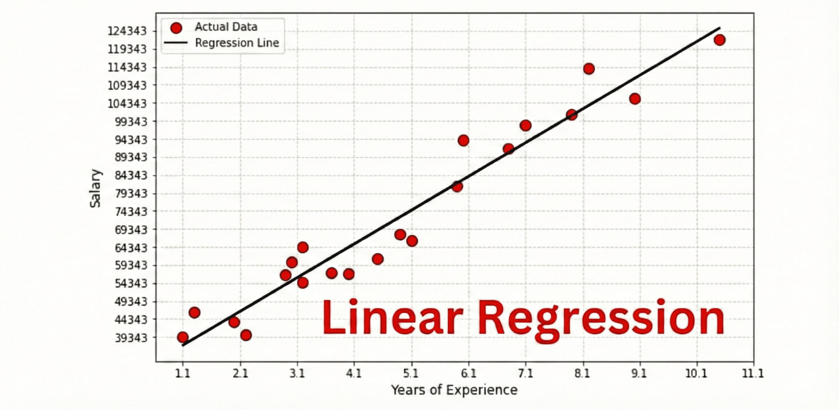
Simple linear regression is a statistical method for finding a linear relationship between two continuous variables. This method is very popular in various fields such as economics, finance, biology, psychology, and engineering. In this article, you will learn various concepts of simple linear regression and its practical implementation in Python using the scikit-learn library.

Assumptions of Simple Linear Regression

A dataset on which we wish to apply simple linear regression should fulfill several assumptions to ensure that the results of the analysis are valid. Let us briefly explain those assumptions one by one:

Linearity: There should be a linear relationship between the independent variable (x) and the dependent variable (y).
Independence: The value of y for different observations should not be related to each other.
Normality: The residual of the data should follow a normal distribution.
Homoscedasticity: The variance of the residuals should be constant across all levels of the independent variables.

Understanding The Mathematics Of Simple Linear Regression

Before applying linear regression, we need to have a basic understanding of the mathematics behind linear regression. This will allow us to gain deeper insight into how the model works, how to interpret the results, and how to identify potential problems.

At its core, a simple linear regression algorithm tries to find a linear relationship between a dependent variable (the one being predicted) and the independent variable (the predictor).

The relationship between the independent variable (x) and the dependent (y) in simple linear regression can be expressed as,

$y^p=b_0+b_1x$

In the above equation, x is the independent variable, yp is the predicted value of the dependent variable y, b0 is the intercept, and b1 is the slope of the line.

The goal of simple linear regression is to find a line (best-fit line) that fits the scattered data (x, y) in the best way by finding the appropriate value of the parameters (slope and intercept) of the above equation.

The appropriate values of the parameters can be evaluated by minimizing the squared difference between the observed value and the predicted value of the dependent variable.

$\min F = \sum_i^n \left(y_i^0 – y_i^p\right)^2$

Figure 1 shows a pictorial representation of linear regression.

$Visualizing The Mathematics Of Simple Linear Regression$

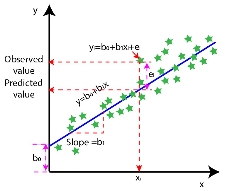
Figure 1: Visualizing the mathematics of simple linear regression

Now that we have covered the basic intuition and math, let us implement simple linear regression in Python.

Practical Implementation Of Simple Linear Regression with scikit-learn

Scikit-learn is a popular Python library that can be used to build and analyse machine-learning models. It contains various algorithms for classification, regression, clustering, and dimensionality reduction. Scikit-learn also offers data preprocessing methods such as feature scaling, encoding categorical variables, and handling missing values.

Let us explore simple linear regression with the help of a practical example in Python using the scikit–learn module.

We have a dataset that contains a collection of data points representing the salary of individuals based on their experience. We will use this dataset to build and evaluate a simple linear regression model to effectively capture the relationship between the independent and dependent variables in the dataset. For a better understanding, we can refer to the table below (Figure 2):

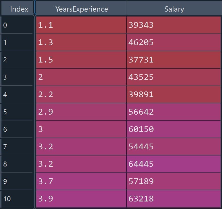
Dataset for simple linear regression example

Figure 2: Dataset for simple linear regression example

Import Necessary Libraries

We will start by importing the libraries we will use throughout this example. NumPy helps with numerical operations, Pandas helps us load and work with the dataset, and Matplotlib is used to visualize the results.

import numpy as np
import pandas as pd
import matplotlib.pyplot as plt

Import Datasets

Next, we will load the CSV file using Pandas. Here, X represents the independent variable (experience) and y represents the dependent variable (salary).

data = pd.read_csv('Experience_Salary_Data.csv')
X = data.iloc[:, :-1].values
y = data.iloc[:, -1].values

Splitting Datasets in Training and Testing Sets

Next, we will split the dataset into a training set and a testing set. The model learns the relationship from the training data, and we use the test data to check how well it generalizes to unseen examples.

from sklearn.model_selection import train_test_split
X_train, X_test, y_train, y_test = train_test_split(X, y, test_size = 0.3, random_state = 0)

Train A Linear Regression Model

Now, we will create a linear regression model and fit it to the training data.

from sklearn.linear_model import LinearRegression
regressor = LinearRegression()
regressor.fit(X_train, y_train)

Model Prediction

Once the model is trained, we can use it to predict salaries for the test set.

y_pred = regressor.predict(X_test)

Visualizing Regression Results (Training Datasets)

The plot below shows the regression line fitted on the training data.

plt.scatter(X_train, y_train, color = 'red')
plt.plot(X_train, regressor.predict(X_train), color = 'blue')
plt.title('Salary vs Experience (Training set)')
plt.xlabel('Years of Experience')
plt.ylabel('Salary')
plt.show()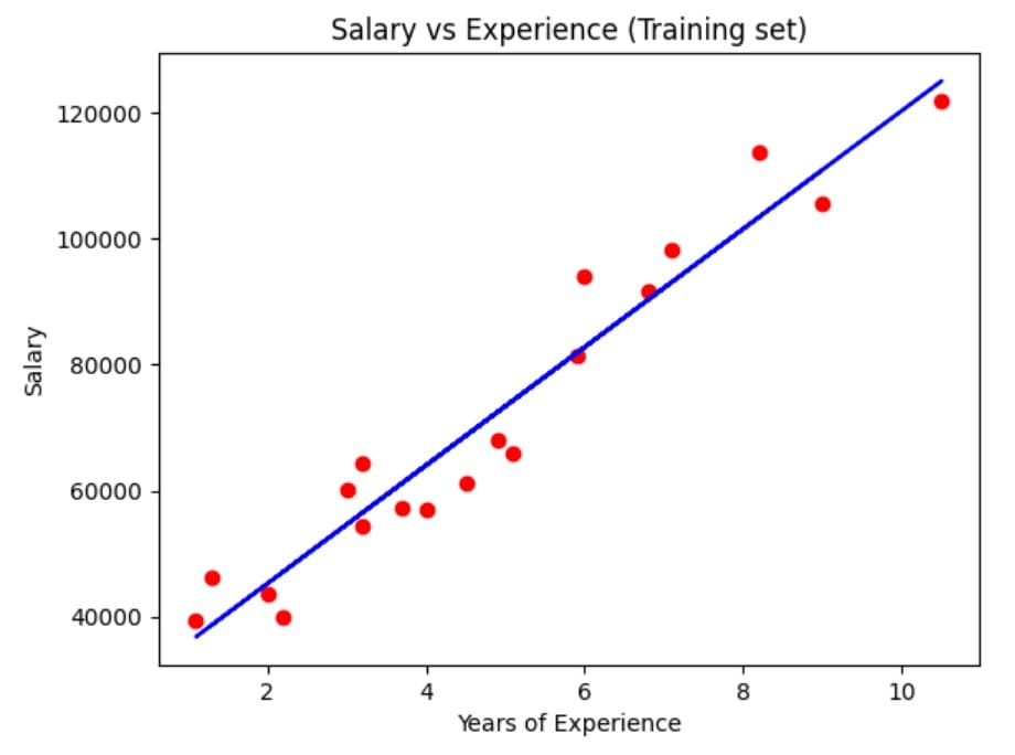

Regression plot on training data

Figure 3: Regression plot on training data

Visualizing Regression Results (Test Datasets)

Similarly, we can visualize how the same regression line compares against the test data.

plt.scatter(X_test, y_test, color='red', marker='o')
plt.plot(X_train, regressor.predict(X_train), color='blue')
plt.title('Salary vs Experience (Test set)')
plt.xlabel('Years of Experience')
plt.ylabel('Salary')
plt.show()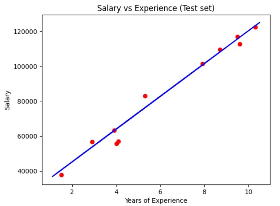

Regression plot on test data

Figure 4: Regression plot on test data

Calculate R-squared score

Finally, we will evaluate the model. The R-squared score indicates how much of the variance in the dependent variable is explained by the model (higher is better).

# Calculate R-squared score
from sklearn.metrics import mean_absolute_error, mean_squared_error, r2_score
y_predict=regressor.predict(X_test)
r2 = r2_score(y_test, y_predict)
print("R-squared score: ", r2)

R-squared score:  0.9766870911747516

We can also compute common error metrics such as MAE, MSE, and RMSE to quantify the average prediction error.

from sklearn.metrics import mean_absolute_error,mean_squared_error
y_predict=regressor.predict(X_test)
MAE = mean_absolute_error(y_test,y_predict)
MSE = mean_squared_error(y_test,y_predict)
RMSE = np.sqrt(MSE)
print("MAE:",MAE )
print("MSE:",MSE )
print("RMSE:",RMSE )

Common Challenges And Pitfalls In Simple Linear Regression

Simple linear regression assumes linear relationships between the dependent variable and the independent variable. However, real-world problems usually show non-linear relationships between variables. For such cases, the use of linear regression may lead to inaccurate results.
Another problem with simple linear regression is the assumption of homoscedasticity, which means that the variance of the errors is constant across all levels of the independent variable. However, violation of these assumptions can lead to inaccurate estimates of regression coefficients and incorrect inferences.
Another pitfall of simple linear regression is multicollinearity which occurs when two or more independent variables are highly correlated. It is difficult to interpret the relationship between dependent and independent variables when multicollinearity exists. Moreover, multicollinearity may lead to unstable estimates of regression coefficients.
In simple linear regression, overfitting is another issue that happens when the model fits the training data very well but cannot properly generalize unseen new data. We can avoid overfitting by various techniques such as cross-validation, regularization, and reducing the number of independent variables.

Conclusions

In this article, we discussed the fundamentals of simple linear regression. We started with an overview of the topic and then discussed various assumptions of simple linear regression. We also learned how to apply simple linear regression with practical implementation in Python using scikit-learn.

We observed that simple linear regression is a powerful tool for modeling linear relationships between dependent and independent variables. Simple linear regression can be used in various fields such as finance, economics, and engineering. An understanding of the assumptions and mathematics of simple linear regression can help us to create accurate models that may facilitate better decision-making.

Frequently Asked Questions

What is meant by simple linear regression?

Simple linear regression is a statistical method used to find the relationship between a dependent variable and an independent variable by fitting a straight line that best describes this relationship.

How to interpret simple linear regression?

Simple linear regression represents a linear relationship between an independent variable and a dependent variable. From this relationship, we can interpret how changes in the independent variable affect the dependent variable. The R-squared value helps us further evaluate the model's performance in fitting the relationship between the dependent and independent variables.

Is simple linear regression the same as correlation?

No, simple linear regression and correlation are not the same.

Simple linear regression involves fitting a model to approximate the relationship between an independent and dependent variable. The model computes the slope and intercept of a line. We can use the model to predict and understand the relationship between the variables.

On the other hand, correlation is used to measure the strength and direction of the linear relationship between two variables using a coefficient ranging from -1 to 1. It does not involve making predictions or calculating a regression line.